We have already highlighted the basic principle of LIBS in our previous blog article. To analyse the plasma, we split up its radiation into thousands of different wavelengths and measure them at the same time. This super-fine spectral resolution enables identification of ‘line emissions’ – sharp peaks in the spectrum caused by various chemical elements in the plasma. You can see several spectra with such peaks in the figure below. The non-linear interactions between the different elements can make the interpretation of spectra difficult. This is where artificial intelligence (AI) and here more specifically machine learning (ML) can help us in classifying the spectra into different groups of materials.

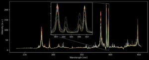
Figure 1: Several raw LIBS spectra, each line colour representing a different refractory material. The zoomed-in section shows four peaks with the two central peaks indicating aluminium, the outer two peaks indicating calcium. The different ratios of areas under each peak allow the identification of the material.

Collecting lots of data is straightforward but analysing it in real-time can quickly become challenging. The most basic approach is to input the entire spectrum with its thousands of channels into a ML model. The computer would then calculate patterns and correlations in the data which are related with the material class on a purely statistical basis. However, this will likely result in a very big and complex model with long computation time. To train the model you’d need lots and lots of data for the model to have a chance of identifying the important features.

A smarter way is to do a feature selection beforehand, so you pass only the information-rich features on to your model. One common way is doing a principal component analysis (PCA), which essentially projects the spectral data onto just a few channels while retaining as much variance of the data as possible. However, the inherent noise within the spectra, which is always present but not related to the material, spoils this approach. Instead, what is usually done with LIBS spectral data is integrating the energy within certain spectral bands, so called regions-of-interest (ROI). This method effectively averages out most of the noise. While there are some AI-based approaches to select these ROI automatically, in most cases a manual selection still wins. Here a PCA can refine this manual selection by reducing it to a few features with low collinearity, which is advantageous for ML.

Now on to the choice of a ML architecture which will allow us to identify the material of a sample. This is usually highly dependent on the task and data on hand. As ML is still a relatively new field in science, choosing the right architecture can be more of an art than science, which requires experience and some good guesses. One constant challenge is finding the best balance between your model learning the fine details of the data, while not faultily learning the random noise as well. You do this by dividing up your data into a training set and a test set. The training set you use to adjust the model parameters, so it classifies the training data as best as possible. You do this multiple times while testing different architectures. Finally, you evaluate which model performs best with the still unused test set, therefore testing how well your model can predict from yet unseen data. A result of such a test is shown in the figure below.

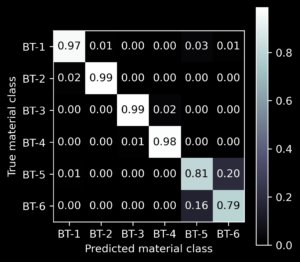
Figure 2: Classifier performance when predicting the class from 3 different, yet unseen, measurements. The table shows, by the value in the upper left cell, that 97 % of the measurements predicted as class BT-1 were really originating from material BT-1, whereas 2 % were originating from material BT-2 (cell below). This model was already very good at classifying the classes BT-1 to BT-4, but there are still difficulties to distinguish BT-5 and BT-6. Therefore, the architecture and training of the model is adapted for further improvement.

This ML-based approach has another advantage over traditional solutions. While calculating the ROI values gets rid of most of the noise, there is still a significant amount present. To mitigate this, it’s possible to average over multiple measurements of the same sample. Of course, this comes with the cost of a slower measurement rate. The ML-based approach offers a better generalisation, meaning it more effectively ignores noise. This allows prediction from a single measurement already, or through combinatorial statistics, a very reliable prediction from multiple measurements.